This microsite is associated to the paper

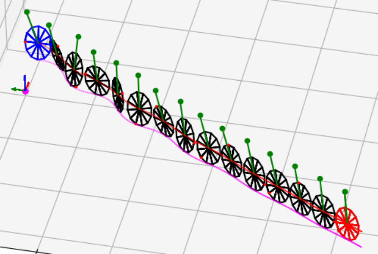
L. Jaulin (2023). Modelisation and control of the rodwheel

Sympy Code to generate the symbolic functions used inside the state space model

from sympy import *
import dill
dill.settings['recurse'] = True

t = symbols('t')
m,g,r,μ,l= symbols('m g r μ l')
c1,c2 = Function('c1')('t'),Function('c2')('t')
dc1,dc2 = Function('dc1')('t'),Function('dc2')('t')
ddc1,ddc2 = Function('ddc1')('t'),Function('ddc2')('t'),
ψ,θ,φ,β = Function('ψ')('t'),Function('θ')('t'),Function('φ')('t'),Function('β')('t')
dψ,dθ,dφ,dβ = Function('dψ')('t'),Function('dθ')('t'),Function('dφ')('t'),Function('dβ')('t')
ddψ,ddθ,ddφ,ddβ = Function('ddψ')('t'),Function('ddθ')('t'),Function('ddφ')('t'),Function('ddβ')('t')
λ1,λ2 = Function('λ1')('t'),Function('λ2')('t')

def subsdiff(E):
    for i in range(0,2):
        E=E.subs({diff(dc1,t): ddc1,diff(dc2,t): ddc2,  diff(dφ,t): ddφ, diff(dθ,t): ddθ, diff(dψ,t): ddψ,diff(dβ,t): ddβ})
        E=E.subs({diff(c1,t): dc1,diff(c2,t): dc2,  diff(φ,t): dφ, diff(θ,t): dθ,diff(ψ,t): dψ, diff(β,t): dβ})
    return simplify(E)

def Rφθψ(φ,θ,ψ):
    Rφ = Matrix([ [1,0,0],[0,cos(φ),-sin(φ)],[0,sin(φ),cos(φ)]])
    Rθ = Matrix([ [cos(θ),0,sin(θ)],[0,1,0],[-sin(θ),0,cos(θ)]])
    Rψ = Matrix([ [cos(ψ),-sin(ψ),0],[sin(ψ),cos(ψ),0],[0,0,1]])
    return Rψ*Rθ*Rφ

def Lagrangian(q,dq):
    c1,c2,φ,θ,ψ,β=list(q)
    dc1,dc2,dφ,dθ,dψ,dβ=list(dq)
    R = Rφθψ(φ,θ,ψ)
    W=simplify(Transpose(R)*diff(R,t))
    wr=Matrix([[-W[1,2]],[W[0,2]],[-W[0,1]]])
    c3=r*cos(θ)
    dc3=diff(c3,t)
    s=Rφθψ(β,θ,ψ)*Matrix([[0],[0],[l]])+Matrix([[c1],[c2],[c3]])
    ds=diff(s,t)
    Ep=m*g*c3+μ*s[2]
    I=Matrix([[1/2*m*r**2,0,0],[0,1/4*m*r**2,0],[0,0,1/4*m*r**2]])
    Ek=1/2*m*(dc1**2+dc2**2+dc3**2)+1/2*μ*(ds[0]**2+ds[1]**2+ds[2]**2)+(1/2)*wr.dot(I*wr)
    L=subsdiff(Ek-Ep)
    return Matrix([L])


q=Matrix([c1,c2,φ,θ,ψ,β])
dq=Matrix([dc1,dc2,dφ,dθ,dψ,dβ])
ddq=Matrix([ddc1,ddc2,ddφ,ddθ,ddψ,ddβ])


L=Lagrangian(q,dq)
Q=subsdiff(diff(L.jacobian(dq),t)-L.jacobian(q))
A=Matrix([[1,0,-r*sin(ψ),-r*cos(ψ)*cos(θ),r*sin(ψ)*sin(θ), 0],
          [0,1, r*cos(ψ),-r*sin(ψ)*cos(θ),-r*cos(ψ)*sin(θ), 0]])
τ=λ1*A[0,:]+λ2*A[1,:]
a=A*dq
da=diff(a,t)
da=subsdiff(da)
S=Matrix([da,*list(Q-τ)])
M=S.jacobian([λ1,λ2,ddq])
M=simplify(M)
b=-S.subs({λ1:0,λ2:0,ddc1:0,ddc2:0,ddφ:0,ddθ:0,ddψ:0,ddβ:0})
b=simplify(b)

F=lambdify((c1,c2,φ,θ,ψ,β,dφ,dθ,dψ,dβ,m,g,r,μ,l),(dc1-a[0],dc2-a[1],dφ,dθ,dβ,dψ,M,b))
dill.dump(F, open("rodwheel.dat", "wb"))

Code for the simulation and control of the rodwheel

import dill
dill.settings['recurse'] = True


def f(x,u):
    dc1,dc2,dφ,dθ,dψ,dβ,M,b=symb(*list(x.flatten()),m,g,r,μ,l)
    bu=array([[0],[0],[0],[0],[1],[0],[0],[-1]])
    λddq=np.linalg.solve(M,b+bu*u)
    ddφ,ddθ,ddψ,ddβ=list((λddq[4:8]).flatten())
    return array([[dc1],[dc2],[dφ],[dθ],[dβ],[dψ],[ddφ],[ddθ],[ddψ],[ddβ]])


def control(x):
    c1,c2,φ,θ,ψ,β,dφ,dθ,dψ,dβ=list(x.flatten())
    β0=0.2*tanh(10-dφ)
    u=5*(β-β0)+5*dβ+20*(abs(θ))
    return u

from roblib import *
symb=dill.load(open("rodwheel.dat", "rb"))


def draw_wheel3D(ax,x,y,z,φ,θ,ψ,r=1,col='blue',size=1):
    M=tran3H(x,y,z)@eulerH(φ,θ,ψ)@wheel3H(r)
    draw3H(ax,M,col,False,1)
    p=array([[x],[y],[z]])+eulermat(φ,θ,ψ)@array([[0],[1],[0]])
    ax.scatter(*p,color='red',s=3)

def draw(ax,x,r,l,col):
    c1,c2,φ,θ,ψ,β,dφ,dθ,dψ,dβ=list(x.flatten())
    w=array([[cos(θ)*cos(ψ),-sin(ψ),0],[cos(θ)*sin(ψ),cos(ψ),0],[-sin(θ),0,1]]@array([[dφ],[dθ],[dψ]]))
    c3=r*cos(θ)
    s=array([[c1],[c2],[c3]])+l*array([[sin(β)*sin(ψ) + sin(θ)*cos(β)*cos(ψ)],[-sin(β)*cos(ψ)+sin(θ)*sin(ψ)*cos(β)],[cos(β)*cos(θ)]])
    draw_wheel3D(ax,c1,c2,c3,φ,θ,ψ,r,col)
    ax.scatter(s[0,0],s[1,0],s[2,0],color='green',s=10)
    ax.plot([c1,s[0,0]],[c2,s[1,0]],[c3,s[2,0]],color="green")
    draw_axis3D(ax,0,0,0,eye(3,3))

def SimuRollingDisk(x,xmin,xmax,ymin,ymax,zmin,zmax,tmax):
    ax = Axes3D(figure())
    dt = 0.02
    C1,C2,C3,G1,G2,G3=[],[],[],[],[],[]
    draw(ax,x,r,l,"blue")
    for t in arange(0,10,dt):
        c1,c2,φ,θ,ψ,β,dφ,dθ,dψ,dβ=list(x.flatten())
        if c1**2+c2**2>100:
            x[0,0],x[1,0]=0,0
            C1.clear(); C2.clear(); C3.clear()
            G1.clear(); G2.clear(); G3.clear()

        u=control(x)
        x=x+dt*(0.25*f(x,u)+0.75*(f(x+(2/3)*dt*f(x,u),u)))
        pause(0.001)
        clean3D(ax,xmin,xmax,ymin,ymax,zmin,zmax)
        draw(ax,x,r,l,"black")


m,g,r,μ,l = 5,9.81,1,1,2
c1,c2,φ,θ,ψ,β,dφ,dθ,dψ,dβ= 0,0,0,  0,0,-0.5,6, 0,0,0  
c1,c2,φ,θ,ψ,β,dφ,dθ,dψ,dβ= 0,0,0,0.3,0,-0.5,6,-3,0,0 
xmin,xmax,ymin,ymax,zmin,zmax=-8,8,-8,8,0,16
x=array([[c1],[c2],[φ],[θ],[ψ],[β],[dφ],[dθ],[dψ],[dβ]])
SimuRollingDisk(x,xmin,xmax,ymin,ymax,zmin,zmax,tmax)